4 ALT Conference Prep
If you are attending our workshop at the ALT conference and would like to live-code along with us during the workshop, please complete this set-up chapter in advance so that you have everything you need.
4.1 Installing R and RStudio
If you don't have R and RStudio already installed, please follow the instructions in the appendix then come back to this chapter.
4.2 Workshop prep
If you've worked with R before and have some basic familiarity with how to code in R and how objects and functions work, you should install the packages tidyverse,plotly, scales, and ggpubr then skip to the set-up check at the end of the chapter.
If you're an R novice, you will find it helpful to work through the below before the workshop.
4.3 R and RStudio
R is a programming language that you will write code in and RStudio is an Integrated Development Environment (IDE) which makes working in R easier. Think of it as knowing English and using a plain text editor like NotePad to write a book versus using a word processor like Microsoft Word. You could do it, but it would be much harder without things like spell-checking and formatting and you wouldn't be able to use some of the advanced features that Word has developed. In a similar way, you can use R without R Studio but we wouldn't recommend it. RStudio serves as a text editor, file manager, spreadsheet viewer, and more. The key thing to remember is that although you will do all of your work using RStudio for this workshop, you are actually using two pieces of software which means that from time-to-time, both of them may have separate updates.
4.3.1 RStudio
When you installed R, that gave your computer the ability to process the R programming language, and also installed an app called "R". We will never use that app. Instead, we will use RStudio. RStudio is arranged with four window panes.
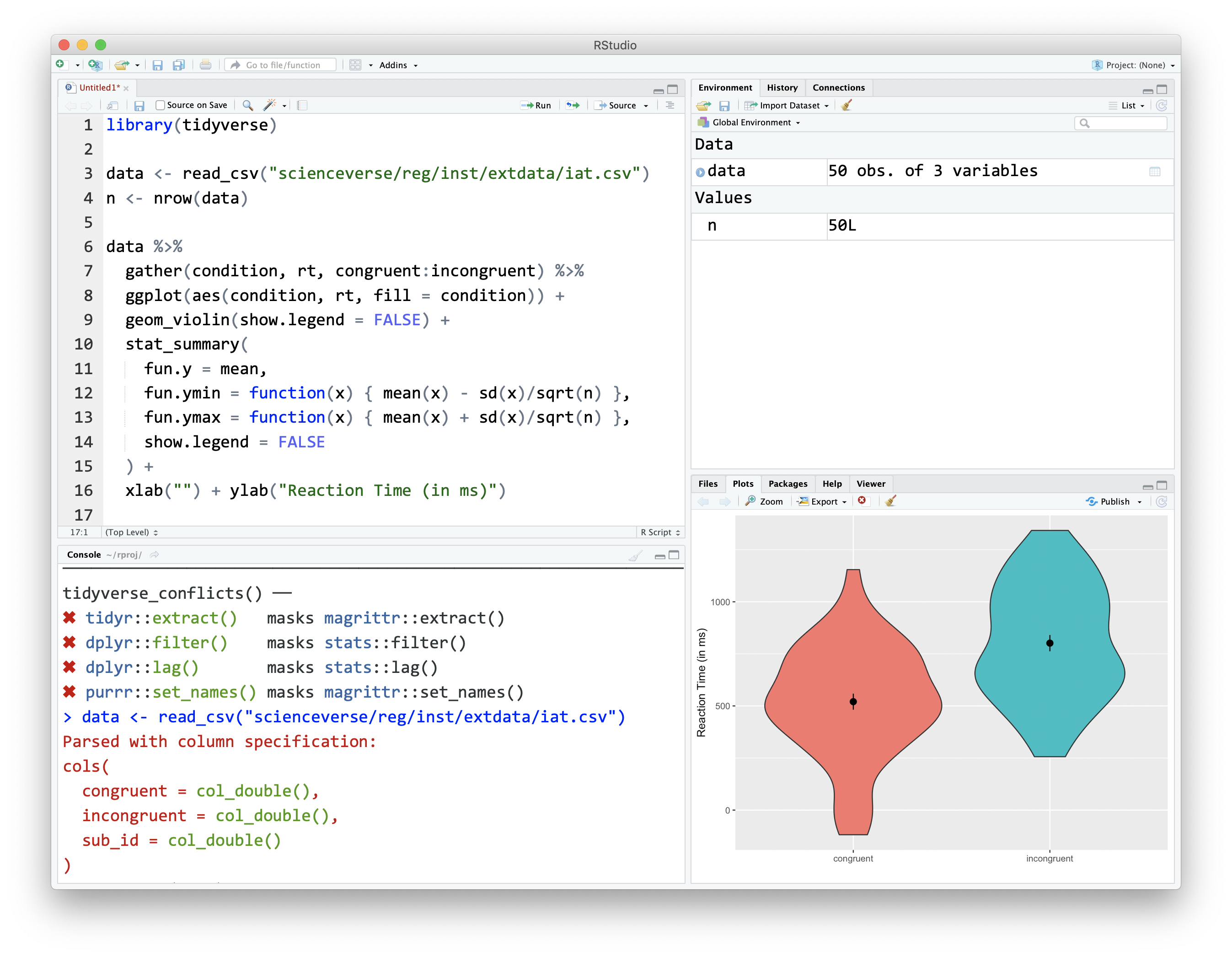
Figure 4.1: The RStudio IDE
By default, the upper left pane is the source pane, where you view, write, and edit code from files and view data tables in a spreadsheet format. When you first open RStudio, this pane won't display until we open a document or load in some data - don't worry, we'll get to that soon.
The lower left pane is the console pane, where you can type in commands and view output messages. You can write code in the console to test it out. The code will run and can create objects in the environment, but the code itself won't be saved. You need to write your code into a script in the source pane to save it.
The right panes have several different tabs that show you information about your code. The most used tabs in the upper right pane are the Environment tab and the Help tab. The environment tab lists some information about the objects that you have defined in your code. We'll learn more about the Help tab in Section ??.
In the lower right pane, the most used tabs are the Files tab for directory structure, the Plots tab for plots made in a script, the Packages tab for managing add-on packages (see Section 4.6), and the Viewer tab to display reports created by your scripts. You can change the location of panes and what tabs are shown under Preferences > Pane Layout.
4.3.2 Reproducibility
One of the main reasons to learn R is that you can create reproducible reports. This involves writing scripts that transform data, create summaries and visualisations, and embed them in a report in a way that always gives you the same results.
When you do things reproducibly, others (and future you) can understand and check your work. You can also reuse your work more easily. For example, if you need to create the same exam board report every semester for student grades, a reproducible report allows you to download the new data and create the report within seconds. It might take a little longer to set up the report in the first instance with reproducible methods, but the time it saves you in the long run is invaluable.
4.4 Sessions
If you have the above settings configured correctly, when you open up RStudio and start writing code, loading packages, and creating objects, you will be doing so in a new session and your Environment tab should be completely empty. If you find that your code isn't working and you can't figure out why, it might be worth restarting your R session. This will clear the environment and detach all loaded packages - think of it like restarting your phone. There are several ways that you can restart R:
- Menu: Session > Restart R
- Cmd-Shift-F10 or Ctl-Shift-F10
- type
.rs.restartR()in the console
4.5 Functions
When you install R you will have access to a range of functions including options for data wrangling and statistical analysis. The functions that are included in the default installation are typically referred to as base R and you can think of them like the default apps that come pre-loaded on your phone.
A function is a name that refers to some code you can reuse. We'll be using functions that are provided in packages, but you can also write your own functions.
If you type a function into the console pane, it will run as soon as you hit enter. If you put the function in a script or R Markdown document in the source pane, it won't run until you run the script, knit the R Markdown file, or run a code chunk. You'll learn more about this in the workshop.
For example, the function sum() is included in base R, and does what you would expect. In the console, run the below code:
sum(1,2,3)## [1] 64.6 Packages
One of the great things about R, however, is that it is user extensible: anyone can create a new add-on that extends its functionality. There are currently thousands of packages that R users have created to solve many different kinds of problems, or just simply to have fun. For example, there are packages for data visualisation, machine learning, interactive dashboards, web scraping, and playing games such as Sudoku.
Add-on packages are not distributed with base R, but have to be downloaded and installed from an archive, in the same way that you would, for instance, download and install PokemonGo on your smartphone. The main repository where packages reside is called CRAN, the Comprehensive R Archive Network.
There is an important distinction between installing a package and loading a package.
4.6.1 Installing a package
This is done using install.packages(). This is like installing an app on your phone: you only have to do it once and the app will remain installed until you remove it. For instance, if you want to use PokemonGo on your phone, you install it once from the App Store or Play Store; you don't have to re-install it each time you want to use it. Once you launch the app, it will run in the background until you close it or restart your phone. Likewise, when you install a package, the package will be available (but not loaded) every time you open up R.
Install the tidyverse package on your system. This package is the main package we will use throughout this book for data wrangling, summaries, and visualisation.
# type this in the console pane
install.packages("tidyverse")
If you get a message that says something like package ‘tidyverse’ successfully unpacked and MD5 sums checked, the installation was successful. If you get an error and the package wasn't installed, check the troubleshooting section of Appendix A.10.
Never install a package from inside a script. Only do this from the console pane.
You can also install multiple packages at once. Here is the command to install all of the packages we'll be using in this workshop.
packages <- c(
  "tidyverse",  # for everything
  "plotly",  # Creates interactive plots
  "ggpubr",   # Builds on ggplot2 to build specific publication ready plots
  "scales" # for plot scales
)

install.packages(packages)
4.6.2 Loading a package
This is done using the library() function. This is like launching an app on your phone: the functionality is only there where the app is launched and remains there until you close the app or restart. For example, when you run library(patchwork) within a session, the functions in the package referred to by plotly will be made available for your R session. The next time you start R, you will need to run library(plotly) again if you want to access that package.
After installing thetidyverse package, you can load it for your current R session as follows:
You might get some red text when you load a package, this is normal. It is usually warning you that this package has functions that have the same name as other packages you've already loaded.
You can use the convention package::function() to indicate in which add-on package a function resides. For instance, if you see readr::read_csv(), that refers to the function read_csv() in the readr add-on package. If the package is loaded using library(), you don't have to specify the package name before a function unless there is a conflict (e.g., you have two packages loaded that have a function with the same name).
4.7 Using functions
4.7.1 Arguments
Most functions allow/require you to specify one or morearguments. These are options that you can set. You can look up the arguments/options that a function has by using the help documentation. Some arguments are required, and some are optional. Optional arguments will often use a default (normally specified in the help documentation) if you do not enter any value.
As an example, look at the help documentation for the function sample() which randomly samples items from a list.
?sampleThe help documentation for sample() should appear in the bottom right help panel. In the usage section, we see that sample() takes the following form:
sample(x, size, replace = FALSE, prob = NULL)In the arguments section, there are explanations for each of the arguments. x is the list of items we want to choose from, size is the number of items we want to choose, replace is whether or not each item may be selected more than once, and prob gives the probability that each item is chosen. In the details section it notes that if no values are entered for replace or prob it will use defaults of FALSE (each item can only be chosen once) and NULL (all items will have equal probability of being chosen). Because there is no default value for x or size, they must be specified otherwise the code won't run.
Let's try an example and just change the required arguments to x and size to ask R to choose 5 random letters (letters is a built-in vector of the 26 lower-case Latin letters).
sample(x = letters, size = 5)## [1] "z" "v" "y" "w" "j"sample() generates a random sample. Each time you run the code, you'll generate a different set of random letters (try it). The function set.seed() controls the random number generator - if you're using any functions that use randomness (such as sample()), running set.seed() will ensure that you get the same result (in many cases this may not be what you want to do). To get the same numbers we do, run set.seed(1242016) in the console, and then run sample(x = letters, size = 5) again.
Now we can change the default value for the replace argument to produce a set of letters that is allowed to have duplicates.
## [1] "t" "k" "j" "k" "m"This time R has still produced 5 random letters, but now this set of letters has two instances of "k". Always remember to use the help documentation to help you understand what arguments a function requires.
4.7.2 Argument names
In the above examples, we have written out the argument names in our code (i.e., x, size, replace), however, this is not strictly necessary. The following two lines of code would both produce the same result (although each time you run sample() it will produce a slightly different result, because it's random, but they would still work the same):
Importantly, if you do not write out the argument names, R will use the default order of arguments. That is for sample it will assume that the first value you enter is x. the second value is size and the third value is replace.
If you write out the argument names then you can write the arguments in whatever order you like:
sample(size = 5, replace = TRUE, x = letters)When you are first learning R, you may find it useful to write out the argument names as it can help you remember and understand what each part of the function is doing. However, as your skills progress you may find it quicker to omit the argument names and you will also see examples of code online that do not use argument names, so it is important to be able to understand which argument each bit of code is referring to (or look up the help documentation to check).
In this workshop, we will always write out the argument names the first time we use each function. However, in subsequent uses they may be omitted.
4.7.3 Tab auto-complete
One very useful feature of R Studio is tab auto-complete for functions (see Figure 4.2). If you write the name of the function and then press the tab key, R Studio will show you the arguments that function takes along with a brief description. If you press enter on the argument name it will fill in the name for you, just like auto-complete on your phone. This is incredibly useful when you are first learning R and you should remember to use this feature frequently.
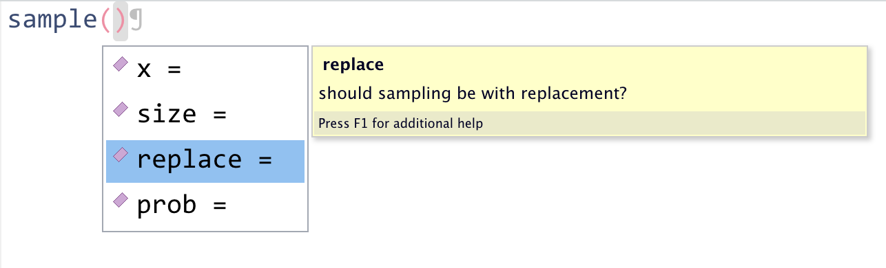
Figure 4.2: Tab auto-complete
4.8 Objects
A large part of your coding will involve creating and manipulating objects. Objects contain stuff. That stuff can be numbers, words, or the result of operations and analyses. You assign content to an object using <-.
Run the following code in the console, but change the values of name and age to your own details and change christmas to a holiday or date you care about.
You'll see that four objects now appear in the environment pane:
-
nameis character (text) data. In order for R to recognise it as character data, it must be enclosed in double quotation marks" ". -
ageis numeric data. In order for R to recognise this as a number, it must not be enclosed in quotation marks. -
todaystores the result of the functionSys.Date(). This function returns your computer system's date. Unlikenameandage, which are hard-coded (i.e., they will always return the values you enter), the contents of the objecttodaywill change dynamically with the date. That is, if you run that function tomorrow, it will update the date to tomorrow's date. -
christmasis also a date but it's hard-coded as a very specific date. It's wrapped within theas.Date()function that tells R to interpret the character string you provide as date rather than text.
To print the contents of an object, type the object's name in the console and press enter. Try printing all four objects now.
Finally, a key concept to understand is that objects can interact and you can save the results of those interactions in new object. Edit and run the following code to create these new objects, and then print the contents of each new object.
decade <- age + 10
full_name <- paste(name, "Nordmann")
how_long <- christmas - today
4.9 Getting help
You will feel like you need a lot of help when you're starting to learn. This won't really go away; it's impossible to memorise everything. The goal is to learn enough about the structure of R that you can look things up quickly. This is why we'll introduce specialised jargon in the glossary; it's easier to google "convert character to numeric in R" than "make numbers in quotes be actual numbers not words". In addition to the function help described above, here's some additional resources you should use often.
4.9.1 Package reference manuals
Start up help in a browser by entering help.start() in the console. Click on "Packages" under "Reference" to see a list of packages. Scroll down to the readxl package and click on it to see a list of the functions that are available in that package.
4.9.2 Googling
If the function help doesn't help, or you're not even sure what function you need, try Googling your question. It will take some practice to be able to use the right jargon in your search terms to get what you want. It helps to put "R" or "tidyverse" in the search text, or the name of the relevant package, like ggplot2.
4.9.3 Vignettes
Many packages, especially tidyverse ones, have helpful websites with vignettes explaining how to use their functions. Some of the vignettes are also available inside R. You can access them from a package's help page or with the vignette() function.
4.10 Workshop set-up check
Restart your R session and then run the below code by copying and pasting it all into the console and then hitting enter. If you have managed to install and update all software and packages as required, it should run without issue and produce the below histograms. It will produce some messages that look like errors involving stat_bin and non-finite values, don't worry, they aren't errors and we'll explain what these messages mean in the workshop.
library(tidyverse)
library(ggpubr)

# Using ggplot2 to visualize distribution of height
gg_height <- ggplot(starwars, aes(x = height)) +
  geom_histogram(binwidth = 10, fill = "blue", alpha = 0.7) +
  labs(title = "Distribution of Heights of Star Wars Characters", x = "Height (cm)", y = "Count")

# Using ggplot2 to visualize distribution of mass
gg_mass <- ggplot(starwars, aes(x = mass)) +
  geom_histogram(binwidth = 10, fill = "red", alpha = 0.7) +
  labs(title = "Distribution of Mass of Star Wars Characters", x = "Mass (kg)", y = "Count")

# Displaying the plots side-by-side using ggpubr
ggarrange(gg_height, gg_mass, ncol = 2, common.legend = TRUE)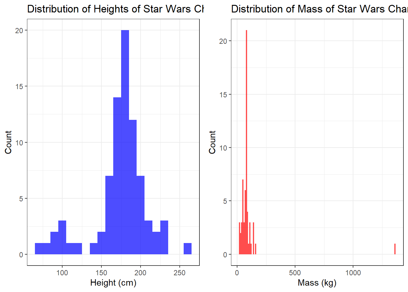
If you get the error there is no package called..., make sure you have installed all the packages listed in Section 4.6.1.
If you are having technical issues working on your own machine and cannot get the below code to run, please use RStudio Cloud for the workshop as there will not be time to troubleshoot installation problems.