6 Exploring Echo360 video/course level data with `tidyverse`

6.1 Introduction

Now we have introduced you to the basic principles of reading and summarising Echo360 data, in this chapter we will explore how you can wrangle and visualise video and course level data to recreate and build on the kind of dashboards you can access on Echo360.

You will need the following packages which are the same as chapter 6, but with the addition of scales to add some useful functions for plotting graph axes. You will also need the data object you created in chapter 6, but you can rerun the code below if you do not have it available already. If you do not have the data downloaded already, please download the .zip file containing 9 files of Echo360 data. Our tutorial assumes you have a folder called "data" in your working directory, and we created a subfolder called "Echo360_Data" to place these files. If you saved the data in another way, remember to edit the file paths first.

library(tidyverse) # Package of packages for plotting and wrangling 
library(plotly) # Creates interactive plots 
library(ggpubr) # Builds on ggplot2 to build specific publication ready plots 
library(scales) # Includes functions for specifying plot scales
library(lubridate)

# Obtain list of files from directory
files <- list.files(path = "data/Echo360_Data/", 
                    pattern=".csv") 

# Read in all files
data <- read_csv(paste0("data/Echo360_Data/", files), # Add our working directory to the list of files 
                 id="video") # What should be call the column containing the name of the video file? 

# Fill in spaces between column names
data <- tibble(data, 
               .name_repair = "universal") # Setting to universal makes all names unique and syntactic

# To break this code down, we start with the innermost function
# 1. We first make each unique video name a factor (unique category)
# 2. We then make each factor a number, so we get an ascending number from 1 to 9
data$video <-as.factor(as.numeric(as.factor(data$video)))

6.2 Handling date/time data with `lubridate`

It's important to be able to track engagment with lecture recordings throughout the semester so being able to analyse the data according to time and data is importnat. Handling date/time data in R is somewhat different from other variable types and should be treated differently and handled with care. The lubridate package in R (loaded as part of the tidyverse) allows us to easily handle tricky date/time data and extract useful information from these.

6.2.1 Converting variables to date/time format

The first task will be to convert any date/time data we have into the correct format. In the sample data we are working with, we have five variables which contain such data which are: Create.Date, Duration, Total.View.Time, Average.View.Time and Last.Viewed.

On closer inspection, these variables fall into two types:

Create.Data and Last.Viewed are listed as a date (a particular day)
Duration, Total.View.Time and Average.View.Time are listed as a time, recorded in hours, minutes, and seconds.

Several functions can be used to take a data string and convert it into the desired date/time format. There is a useful cheat sheet you can download for the lubridate library which contains examples of such functions. For our data, we will use the mdy() function to convert dates as month-day-year, and the hms() function to convert times as hours-minutes-seconds.

# For times, mutate across three columns and convert to hours, minutes, seconds
# For dates, mutate across two columns and convert to month, day, year
data <- data %>%
  mutate(across(.cols = c('duration', 'total_view_time', 'average_view_time'), 
                .fns = hms)) %>%
  mutate(across(.cols = c('create_date', 'last_viewed'), 
                .fns = mdy))

Here, we use a combination of mutate and across to apply a given function to multiple columns. Within across, we specify two arguments. In .cols, we specify the columns we want to apply our function to and in .fns, we specify the function we want to apply to those columns.

hms() converts a string into a date/time object which is set by hours-minutes-seconds. mdy() converts a string into a date/time object which is set by month-day-year. Echo360 data saves date/times in US format, so pay attention to how date/time data is stored to data you work with to make sure it recognises the information in the right order. There are alternative functions like ymd() and dmy() if data you work with is stored differently.

We can take a look at the result of these transformations more closely using head() to preview the first five cases of each variable:

# First five cases of duration 
head(data$duration)
# First five cases of last viewed
head(data$last_viewed)

## [1] "13M 11S" "13M 11S" "13M 11S" "13M 11S" "13M 11S" "13M 11S"
## [1] "2023-01-16" "2023-01-18" "2023-01-24" "2023-01-15" "2023-01-16"
## [6] "2023-02-15"

6.2.2 Transforming time data

To help us summarise and visualise the time data, we can convert time variables to numeric. In this case, we can use mutate() with as.numeric() to convert the variable duration from a time variable (e.g., 13M 11S) to a number (13.2). This then easily allows us to compute summary statistics and visualise the data

# compute mean duration
data %>%
  mutate(duration = as.numeric(duration, "minutes")) %>%
  group_by(video) %>%
  summarise(duration = mean(duration))

# produce bar chart
data %>%
  mutate(duration = as.numeric(duration, "minutes")) %>%
  group_by(video) %>%
  summarise(duration = mean(duration)) %>%
  ggplot(aes(x = video, y = duration, fill = video)) + # fill gives colours for each video
  geom_col() +
  guides(fill = "none") + # removes redundant legend
  theme_minimal() + # apply a theme
  labs(title = "Video length in minutes")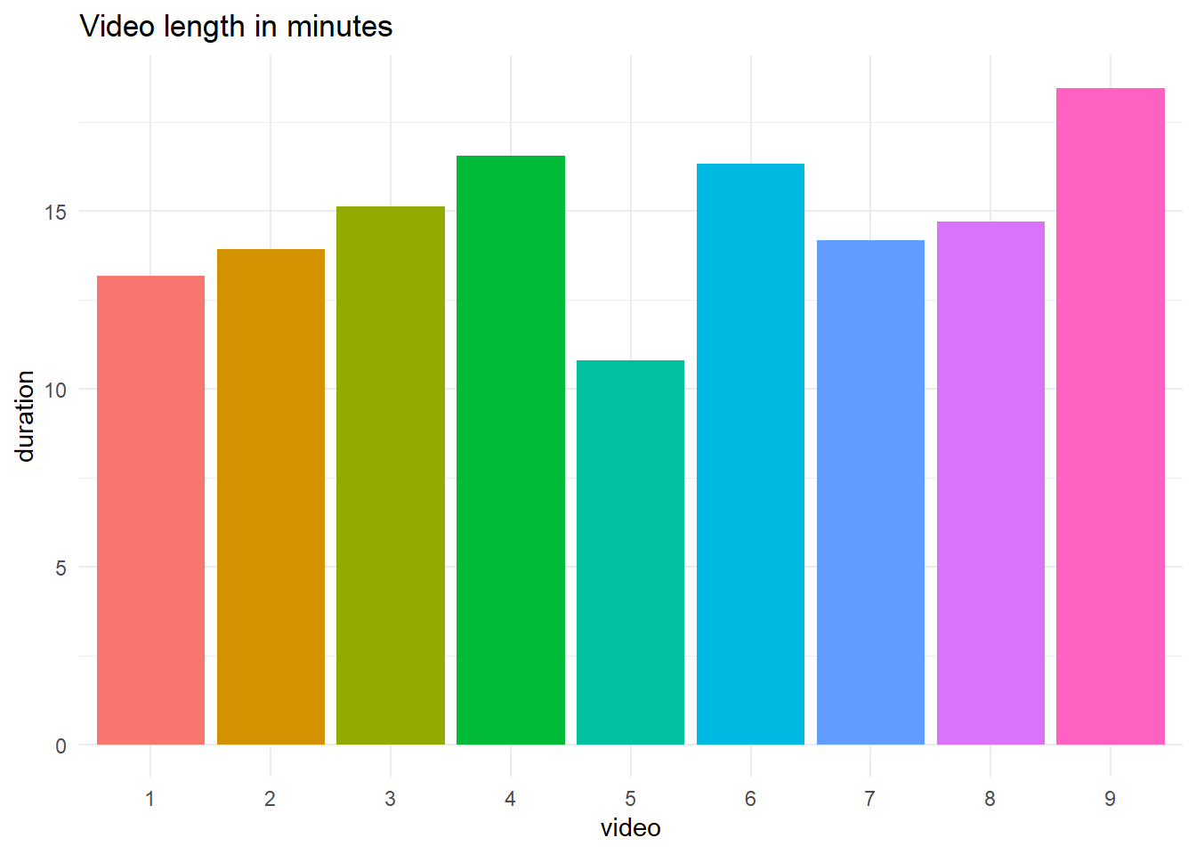

# produce line graph of same data
data %>%
  mutate(duration = as.numeric(duration, "minutes")) %>%
  group_by(video) %>%
  summarise(duration = mean(duration)) %>%
  ggplot(aes(x = video, y = duration, colour = video, group = 1)) + # fill gives colours for each video
  geom_point() +
  geom_line() +
  guides(colour = "none") + # removes redundant legend
  theme_minimal() + # apply a theme
  labs(title = "Video length in minutes") +
  scale_y_continuous(limits = c(0, 20)) #  set limits of y-axis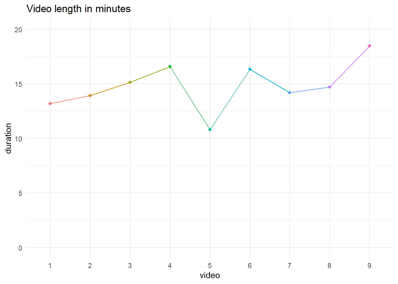

video	duration
1	13.18333
2	13.91667
3	15.13333
4	16.56667
5	10.80000
6	16.33333
7	14.18333
8	14.70000
9	18.46667

6.2.3 Extracting elements from date/time data

Sometimes, you may wish to obtain specific parts of a date/time such as the month, the minutes etc. There are several functions in lubridate which allow us to extract these easily from a date/time object.

Suppose we want to look at the last month students viewed videos across the course. We can obtain this by applying the month() function to the Last.Viewed variable.

# Add a new month column 
data <- data %>% 
  mutate(month_last_viewed = month(data$last_viewed))

last_viewed <- data %>% 
  ggplot(aes(x = month_last_viewed)) + # Only specify x axis for a bar chart
  geom_bar() + # Create a bar chart 
  labs(title = "Frequency of last month video viewed",
       y = "Frequency",
       x = "Last month video viewed") + 
  theme_bw() + 
  scale_x_continuous(breaks = seq(1:12))

last_viewed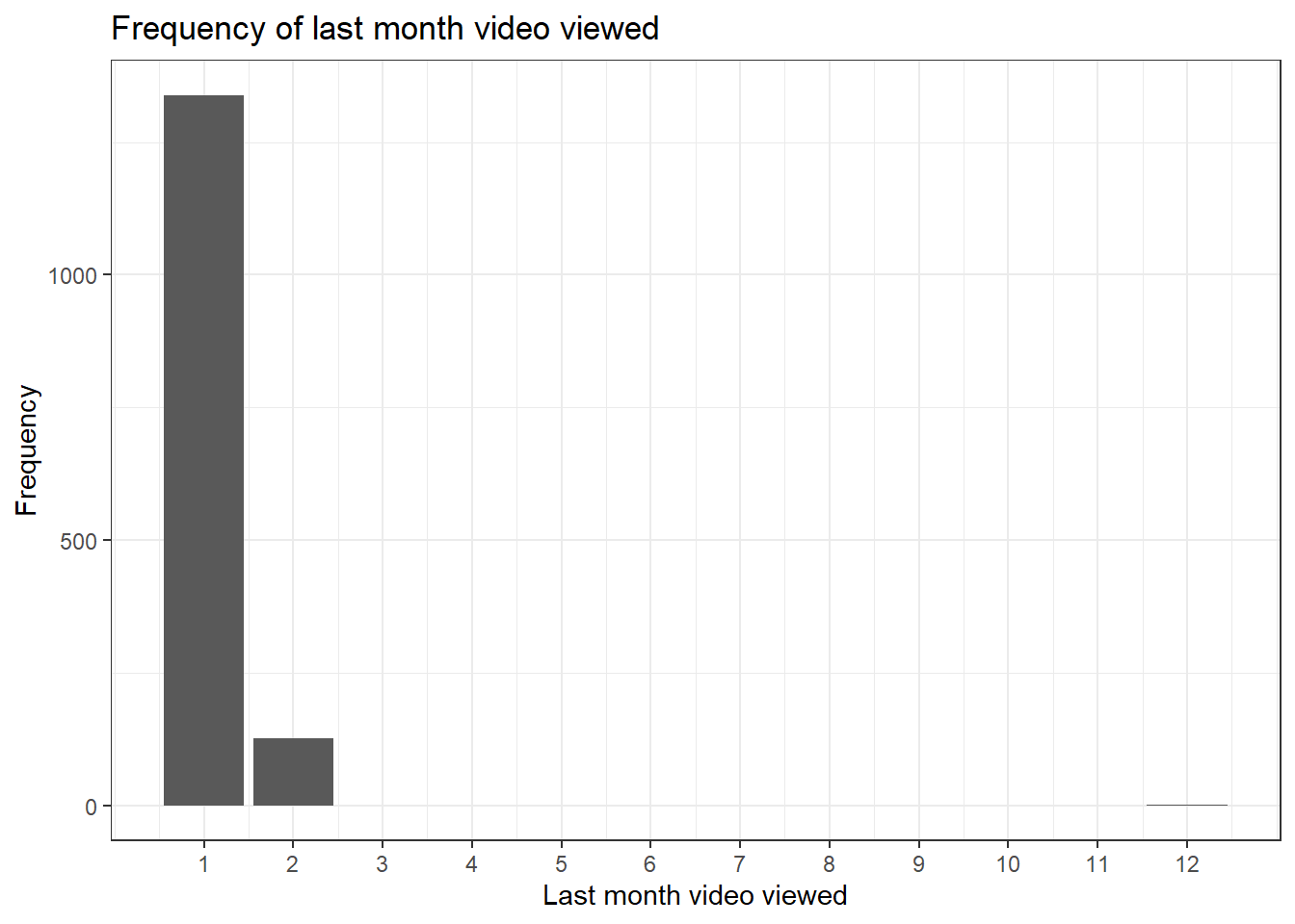

We can also convert the bar chart to make it interactive using the ggplotly() function. This allows you to hover over the plot and see what the frequency was for each month.

ggplotly(last_viewed)

6.2.4 Maths with date-times

Sometimes, we may wish to compare the difference in time between events. lubridate provides some useful functions to help us with this. For example, we can look at the difference in view time to the total duration of the video by using simple arithmetic operators combined with group_by(). As noted, the function of group_by() is that it will perform whatever operation comes after it seperately for each level of the grouping variable so in this case, it will compute the time difference for each video.

data <- data %>% 
  group_by(video) %>%
  mutate(time_difference = average_view_time - duration) %>% # Add a time difference column between average view time and total duration
  ungroup()

head(data$time_difference)

## [1] "-3M 44S"  "-1M 35S"  "-2S"      "-8M 5S"   "-4M 48S"  "-11M -9S"

As this data returns values in minutes and seconds, we can transform this to numeric and create a histogram. More negative values represent students who watched less of the video than the total duration.

data <- data %>% 
  mutate(time_difference = as.numeric(time_difference, "minute"))

time_difference <- data %>% 
  ggplot(aes(x = time_difference)) + 
  geom_histogram() +
  labs(title="Difference between average viewing times & total video duration") +
  theme_bw() 

time_difference

## `stat_bin()` using `bins = 30`. Pick better value with `binwidth`.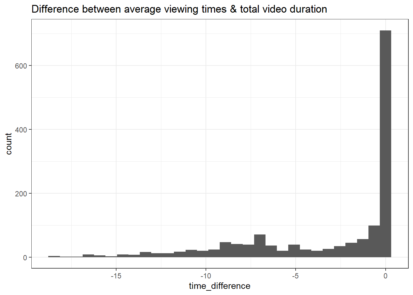

As before, we can make these values interactive by converting our ggplot visualisation to a plotly object.

ggplotly(time_difference)

## `stat_bin()` using `bins = 30`. Pick better value with `binwidth`.

The difference between viewing time and duration is of course relative to the duration so it may be better to express this difference as a percent, i.e., on average, what percent of each video did students watch?

To do this, we can use mutate to calculate the percent of each video viewed. Once we've created this column, we can then use group_by() and ggplot() to summarise and visualise the drop-off for each video.

data <- data %>%
  mutate(percent_watched = 100 - ((duration-average_view_time) / duration) *100) 

data %>%
  group_by(video) %>%
  summarise(mean_percent = mean(percent_watched))


data %>%
  group_by(video) %>%
  summarise(mean_percent = mean(percent_watched)) %>%
  ggplot(aes(x = video, y = mean_percent, colour = video, group = 1)) + # fill gives colours for each video
  geom_point() +
  geom_line() +
  guides(colour = "none") + 
  theme_minimal() + 
  labs(title = "Video length in minutes") +
  scale_y_continuous(limits = c(0, 100)) #  set limits of y-axis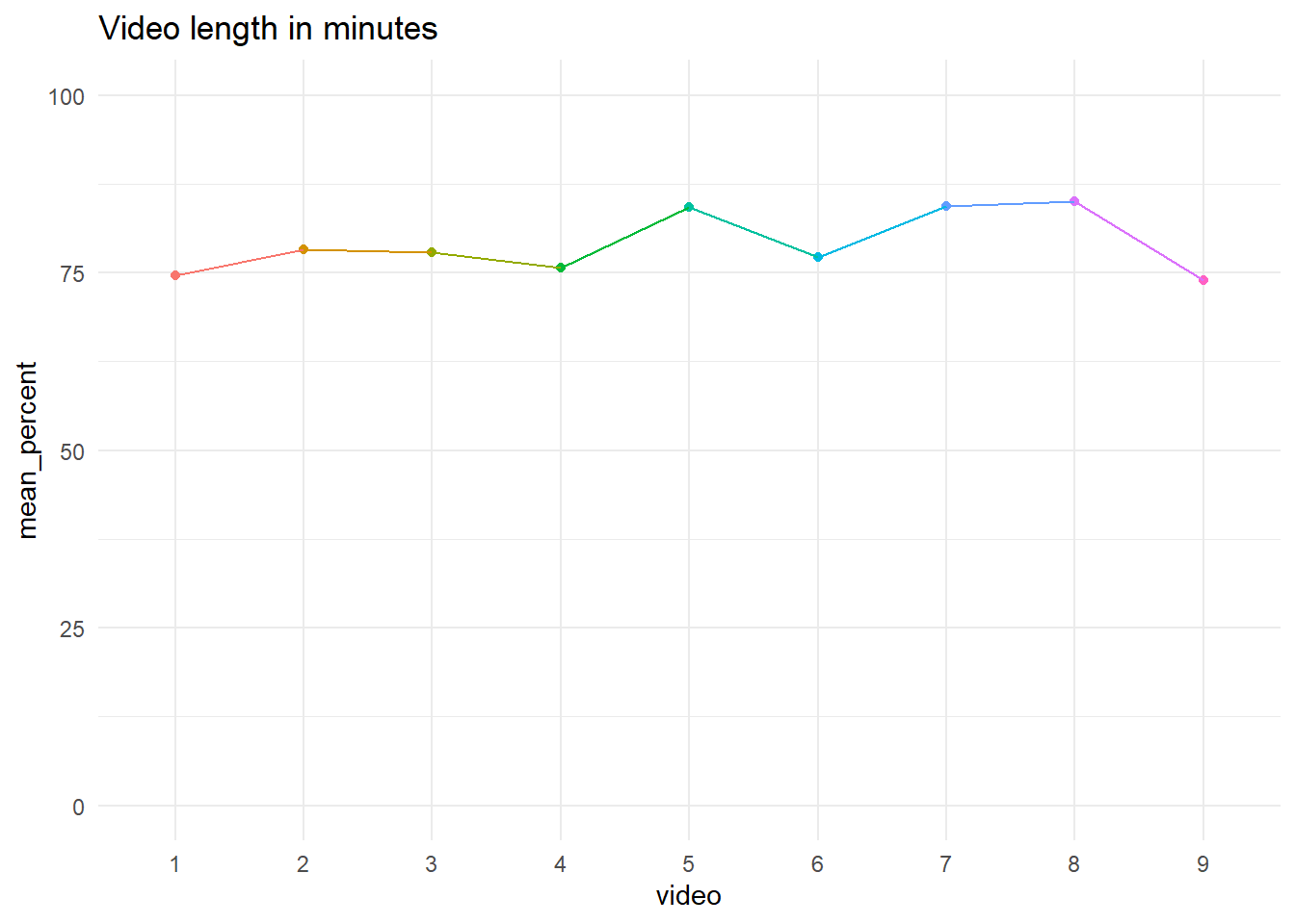

video	mean_percent
1	74.62349
2	78.21563
3	77.84165
4	75.65035
5	84.27152
6	77.16715
7	84.40620
8	85.00724
9	73.96479

6.3 Total views for each video

In the following section, we will continuing creating plots of our data summarised at the video level. Given that our data is currently stored at student level (one row per student per video), we will first transform our data into a new data set called video_data which will group the data by video and create some variables of interest. First, let's create this new data set with two columns:

video: The video number ;
total_views: The total number of views per video.

video_data <- data %>% 
  group_by(video) %>%
  summarise(total_views = sum(total_views)) %>% # for each video, add up all the views across students
  ungroup() # Retaining the group by can sometimes cause problems

We can now easily create a bar chart of the total number of views per video.

fig.total.views <- video_data %>% 
  ggplot(aes(x = video, y = total_views)) +
  geom_col() + 
  labs(title="Total number of views per video",
       y = "Total Views",
       x = "Video") + 
  theme_bw()

fig.total.views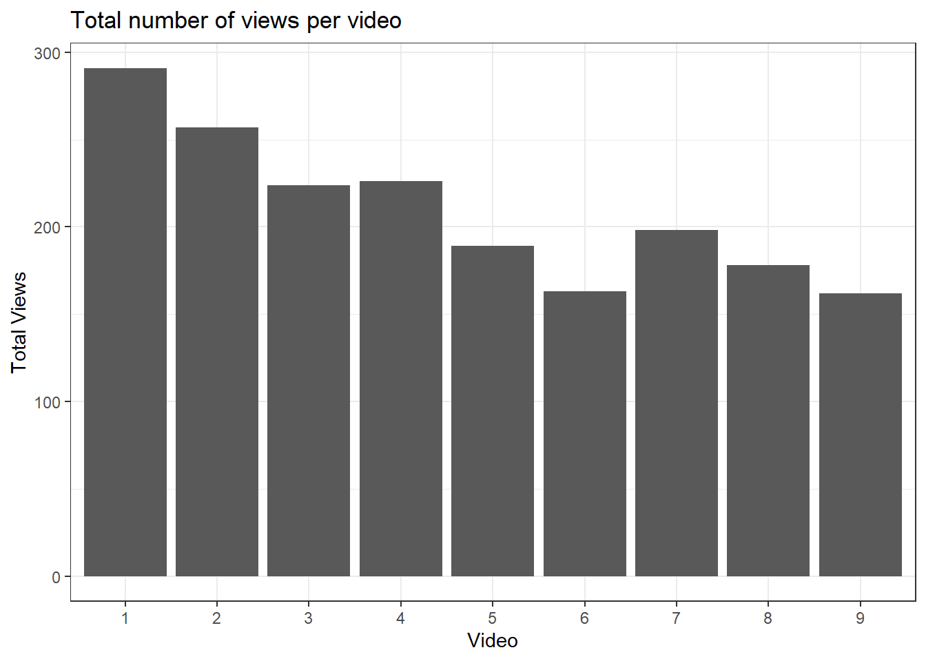

Here, we plot the video number along the x-axis and the total number of views for each video on the y-axis. These numbers include duplications from students who have watched the videos multiple times.

We may also be interested in the total number of unique views, i.e. the total number of students who watched the video at least once. To do this, we need to create a new variable called unique_views which will contain the sum of the rows for each video. We can add this to the video-level data set video_data.

video_data <- data %>% 
  group_by(video) %>%
  summarise(total_Views = sum(total_views), 
            unique_views = n()) %>% # For each video, count the number of rows
  mutate(video = factor(video)) %>% 
  ungroup()

We can edit the code for the previous bar chart to create a bar chart of the total number of unique student views per video as follows.

fig.unique.views <- video_data %>% 
  ggplot(aes(x = video, y = unique_views)) +
  geom_bar(stat = "identity") + # Since we specify a y value, just show as the value
  labs(title="Total number of unique student views per video",
       y = "Unique Student Views",
       x = "Video") + 
  theme_bw()

fig.unique.views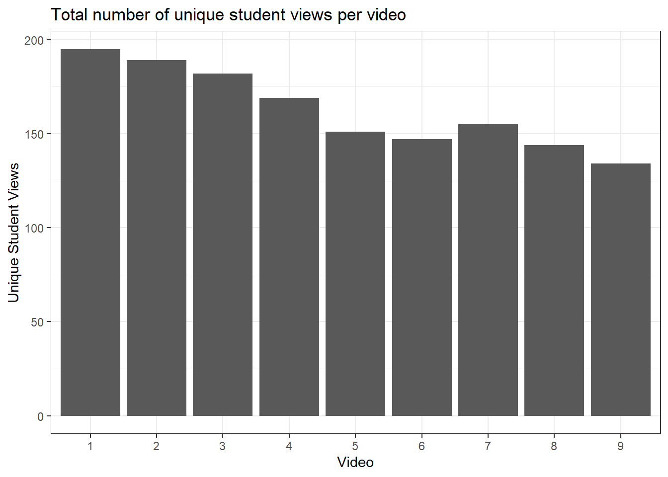

If you want to view the values per video more precisely like a data dashboard, then you can convert your unique views bar plot into a plotly object.

ggplotly(fig.unique.views)

6.3.1 Advanced `plotly` customisation

So far, we have simply transformed our ggplots into a plotly object. However, we can add additional information in the hover text such as total views, duration of video, and average view time that might be useful to you or your viewer.

This is going to be a longer process, so we will break it down into a few steps. First, we need to wrangle the data so we have our key summary statistics per video. The first few lines follow the same process as above, but then we add additional summary variables like the average view time and modify existing variables in mutate().

# Isolate video number and duration of the video to append later
video_duration <- data %>% 
  distinct(video, duration) %>% 
  mutate(duration = period_to_seconds(duration)) # Convert duration from a period to seconds

video_data <- data %>%
  group_by(video) %>%
  summarise(total_views = sum(total_views), 
            unique_views = n(), 
            average_view_time = round(
              mean(period_to_seconds(average_view_time), # lubridate function to transform a period to seconds
                   na.rm = T), # Ignore NA values when taking mean
              0)) %>% # 0 decimals to round
  left_join(video_duration, # Add video duration data to our summary data
            by = "video") %>% # Join by video number
  mutate(video = factor(video),
         repeated_views = total_views - unique_views, # Calculate repeated views subtracting unique views from total views
         percentage_viewed = round(average_view_time / duration * 100, 2)) %>% # Calculate average percentage from average view time as percentage of duration
  ungroup()

head(video_data)

video	total_views	unique_views	average_view_time	duration	repeated_views	percentage_viewed
1	291	195	590	791	96	74.59
2	257	189	653	835	68	78.20
3	224	182	707	908	42	77.86
4	226	169	752	994	57	75.65
5	189	151	546	648	38	84.26
6	163	147	756	980	16	77.14

For each video, we now have a bunch of summary statistics like their view time, duration, and percentage of the video viewed. We can now use this information to present as a dashboard for an overview of each video.

This time, we are going to use plotly directly as its easier to edit the hover text options than if we simply convert a ggplot object to plotly. In the code below, we first create a bar plot for the number of unique views for each video. We then edit the hover template to add additional information into the interactive dashboard like the duration and average view time.

fig.all.views <- plot_ly(video_data,
  x = ~video,
  y = ~unique_views,
  name = "Unique Views",
  type = "bar",
  hovertemplate = paste0("Video %{x}", # Paste adds all the elements together, <br> is html code for a line break
                         "<br>Total views:", video_data$total_views,
                         "<br>Unique views: %{y}",
                         "<br> Duration: ", seconds_to_period(video_data$duration), # Convert from seconds to minutes and seconds for easier viewing
                         "<br> Average view time: ", seconds_to_period(video_data$average_view_time))) %>%
  layout(title = 'Unique Views per Video', 
         xaxis = list(title = 'Video Number'),
         yaxis = list(title = 'Unique Views'))

fig.all.views

Like ggplot2, once we have defined a plotly object, we can add additional layers. In this example, we might also want to create a stacked bar plot with the total number of views split into unique student views and repeated views.

# Take the plotly object and add a trace (variable to split by) for the repeated views
fig.all.views <- fig.all.views %>% 
  add_trace(y = ~repeated_views, 
            name = 'Repeated views') %>% 
  layout(yaxis = list(title = 'Count'), # Amend the type of bar plot to make it stacked
         barmode = 'stack')

fig.all.views

6.4 Video duration vs. average percentage viewed

As one final type of data visualisation, we will create a scatterplot of video duration against the average percentage of video viewed using "ggplot()".

fig.duration.viewed <- video_data %>% 
  ggplot(aes(x = duration, y = percentage_viewed)) +
  geom_point() + 
  labs(title = "Video duration vs. average percentage viewed",
       y = "Average percentage of video viewed",
       x = "Video duration (Seconds)") + 
  theme_bw() + 
  scale_y_continuous(breaks = pretty_breaks()) # Convert the y axis to tidier labels for percentages

fig.duration.viewed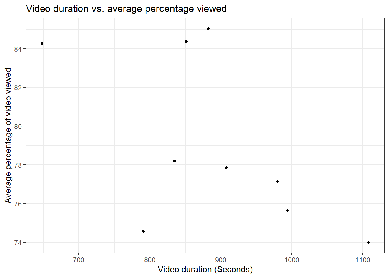

As before, we can convert our scatterplot into a plotly object to make it interactive as we scroll across the values.

ggplotly(fig.duration.viewed)

6.4.1 Advanced `plotly` customisation

Like we demonstrated for the bar plot, we can create a scatterplot entirely within plotly to allow us to modify the hover template to include additional summary statistics.

fig.duration.viewed.2 <- plot_ly(video_data,
               x = ~duration,
               y = ~percentage_viewed,
               type = "scatter",
               mode = "markers",
               hovertemplate = paste0("Video ", video_data$video,
                                      "<br>Average percentage viewed: ", round(video_data$percentage_viewed,1), "%",
                                      "<br> Duration: ", video_data$duration,
                                      "<br> Average view time: ", video_data$average_view_time,
                                      "<extra></extra>"))%>%
  layout(xaxis = list(title = 'Duration of video'),
         yaxis = list(title = 'Percentage of video viewed'))

fig.duration.viewed.2

5 Getting started with Echo360 data with tidyverse

7 Combining Echo360 data with other sources of data with tidyverse

6 Exploring Echo360 video/course level data with tidyverse