2 Creating synthetic datasets

2.1 Introduction

In the scholarship of teaching and learning, we might analyse data from sources like virtual learning environments and student characteristics. Student agreements normally allow educators to analyse these data for the purposes of internally improving education experiences, but if we want to disseminate our findings to a wider audience, we would need to gain ethical approval from the students to use their data for these additional purposes. Even with ethical approval, there might be additional concerns around privacy and anonymity if the data contain sensitive or personal information. As data sharing practices become routine, it is important to contribute to scholarly progress while maintaining participant anonymity. In this tutorial, we will demonstrate how you can create synthetic data sets as a strategy where sharing primary data would present ethical issues.

Synthetic data mimics the properties of your original data as closely as possible, such as retaining the distribution of grades in your sample. This means that we can retain the underlying statistical properties between variables, but "individual participants" would no longer represent the original cases, meaning the risk of identification is much lower. The R package synthpop (Nowok et al., 2016) creates synthetic data by sampling from a probability distribution best suited to the variables in your data set. The precise technical details are beyond the scope of our tutorial, so we refer interested readers to Nowok et al. for further information.

It is important to evaluate each project individually to judge whether you can ethically share research data, but Meyer (2018) provides practical tips:

Wherever possible, get informed consent from participants to retain and share data.
Do not promise to destroy or to never share the data. Often researchers will reassure ethical review boards that the data will never be shared beyond the research team, but providing it would be appropriate to do so, you can simply ask the participants to consent to their data being shared.
Be thoughtful when considering the risks of re-identification.

Assuming you receive consent for data sharing, the likelihood of identifying individual participants motivates our synthetic data tutorial. Even if you exclude identifiable information like names or email addresses, participants could be re-identified through combining common demographic variables such as ethnicity, date of birth, and sex which you might want to share if they are related to your research question. The risk of re-identification may be even higher if participants know each other. For example, students might know you studied their cohort and be able to identify themselves in the data set and recognise other participants relative to their own details. Therefore, if you want to share the data as a part of your scholarship and you receive consent from participants to do so, it is important to think about whether the variables you want to share could be used to identify participants and whether providing a synthetic data set over the original data would be more appropriate. See Meyer (2018) for further details on ethical data sharing.

In this tutorial, we will demonstrate how to create a synthetic data set using the synthpop package in R. Quintana (2020) has previously written an accessible tutorial to the package we recommend but focuses on biomedical science data. Our tutorial will use data on student's academic procrastination to resonate more closely with the scholarship of teaching and learning.

2.1.1 Dunn (2014) Replication

The data set we will use below is from an unpublished replication attempt of Dunn (2014). Dunn wanted to understand the impact of motivation and statistics anxiety on students' academic procrastination. The sample included graduate students on an online only course. We wanted to replicate the study to see if we would observe similar findings in response to the COVID-19 pandemic where face-to-face students were forced to study online. The Dunn replication is perfect to demonstrate a synthetic data set as it includes a range of data types and we included open data in the consent forms, meaning we can openly compare the properties of each data set.

Our research question was: Do intrinsic motivation, academic self-regulation, and statistics anxiety influence students' passive procrastination? We expected intrinsic motivation and self-regulation to be negative predictors, whereas we expected statistics anxiety to be a positive predictor of passive procrastination. The study included the following variables:

General strategies for learning (GSL; GSL) - A modified subscale of the Motivated Strategies for Learning Questionnaire (MSLQ) which measures academic self-regulation. Measured on a 1-7 scale, with higher values meaning higher self-regulation.
Intrinsic motivation (Intrinsic) - A subscale of the MSLQ which measures intrinsic motivation or the inherent joy people find in a task. Measured on a 1-7 scale, with higher values meaning higher intrinsic motivation.
Statistical Anxiety Rating Scale (STARS; STARS) - A measure of statistics anxiety where we only included the statistics test and class anxiety subscale. Measured on a 1-5 scale, with higher values meaning higher statistics anxiety.
Procrastination Assessment Scale for Students (PASS; PASS) - A measure of passive procrastination on keeping up with writing assignments and studying for exams. Measured on a 1-5 scale with higher scores meaning greater procrastination, but this scale uses the sum of items creating a possible range of 6-30.

2.1.2 Prior knowledge

To complete this tutorial you will need the following prior knowledge - recap links point to additional materials that will cover these in more detail):

How to install and load packages in R (recap)
How to set the working directory and run code in R (recap)
How (and why) to use the pipe %>% operator (recap)
A conceptual understanding of linear regression (recap)

2.1.3 Set-up

Before we demonstrate the synthpop package, we will explore the original data set and modelling.

Download Dunn-replication.csv and save it into a folder named data in your working directory.
Then run the below code to load the required packages (may require installation) and data.

library(tidyverse) # Collection of functions for data wrangling and visualisation
library(performance) # Functions for assessing statistical models
library(effectsize) # Functions for calculating effect sizes
library(synthpop) # Package to create our synthetic data set later

# Two functions to make prettier html tables
library(knitr)
library(kableExtra)

real_data <- read_csv("data/Dunn-replication.csv") %>% 
  select(-user_id, -SelfEfficacy, -HelpSeeking) # omit some columns we don't need

2.2 Original dataset analyses

To address our research question using the same model as Dunn (2014), we want to use linear regression with PASS as our outcome and three predictors of GSL, intrinsic motivation, and statistics anxiety.

The function lm() constructs a linear model
The formula takes the form outcome ~ predictor1 + predictor2 etc.
We first save the results of the regression to an object model and then pass this object to the summary() function to explore the model results:

# One outcome, three predictors
model <- lm(PASS ~ GSL + Intrinsic + STARS,
            data = real_data)

(model_results <- summary(model)) # surround with brackets to both print and save

## 
## Call:
## lm(formula = PASS ~ GSL + Intrinsic + STARS, data = real_data)
## 
## Residuals:
##      Min       1Q   Median       3Q      Max 
## -14.8588  -3.4830   0.0803   3.2853   9.9100 
## 
## Coefficients:
##             Estimate Std. Error t value Pr(>|t|)    
## (Intercept)  23.6386     3.0068   7.862  3.2e-12 ***
## GSL          -1.7677     0.4698  -3.762 0.000275 ***
## Intrinsic    -0.1780     0.5160  -0.345 0.730767    
## STARS         1.6926     0.5961   2.840 0.005408 ** 
## ---
## Signif. codes:  0 '***' 0.001 '**' 0.01 '*' 0.05 '.' 0.1 ' ' 1
## 
## Residual standard error: 4.405 on 107 degrees of freedom
## Multiple R-squared:  0.1815, Adjusted R-squared:  0.1586 
## F-statistic: 7.911 on 3 and 107 DF,  p-value: 8.154e-05

For a replication in a different setting, the results are pretty close to Dunn (2014). Overall, we have a significant model which explains 18% (adj. \(R^2\) = 0.16) of the variance in passive procrastination. Similar to Dunn, GSL was a significant negative predictor of passive procrastination, with a 1 unit increase in GSL associated with a 1.77 decrease in passive procrastination. Intrinsic motivation was a non-significant weak negative predictor. Interestingly, statistics anxiety was not a significant predictor for Dunn, but it was a significant positive predictor in our replication, with a 1 unit increase in STARS associated with a 1.69 increase in passive procrastination. In other words, passive procrastination tended to increase with higher levels of statistics anxiety and lower levels of GSL.

These values are in the original units of measurement, but we can also report standardised coefficients to express the values in standard deviations, consistent with how Dunn reported the results. You can do this yourself by standardising the predictors before entering them into the model, or you can use the handy standardize_parameters() function from the effectsize package to get the 95% confidence intervals too. Below, we save the results as a table and add the estimates from Dunn (2014) for comparison.

The below code:

Calculates the standardized coefficients and saves them in an object named table
Creates a vector of the coefficients from the original Dunn study
Adds this vector as a column to table
Makes a nice looking table using kable - note that your table output might look slightly different because the bookdown package we use to write this book applies some additional formatting.

#1. Use the standardize_parameters function
#2. Select rows 2-4, ignoring the intercept
#3. Save in a data frame
#4. Drop the 95% CI column as it's just descriptive 

table <- standardize_parameters(model) %>%
  slice(2:7) %>%
  data.frame() %>%
  select(-CI)

# Manually save values from the original Dunn study for comparison
dunn <- c(-0.55, # GSL
          -0.17, # Intrinsic
          0.15) # STARS

# Add these values to our table above
table$dunn <- dunn

# Use the kable and kableextra functions to create a nicer looking table 
kable(table, 
      digits = 2, 
      format = "html", 
      col.names = c("Parameter", "Beta", "Lower 95% CI", "Upper 95% CI", "Beta from Dunn (2014)"), 
      caption = "Standardised Beta coefficients and their 95% confidence interval (CI) in the replication data compared to Dunn (2014).") %>% 
  kable_styling()

Table 2.1: Standardised Beta coefficients and their 95% confidence interval (CI) in the replication data compared to Dunn (2014).
Parameter	Beta	Lower 95% CI	Upper 95% CI	Beta from Dunn (2014)
GSL	-0.38	-0.58	-0.18	-0.55
Intrinsic	-0.03	-0.23	0.16	-0.17
STARS	0.25	0.08	0.43	0.15

For comparison, our coefficient for STARS was larger than Dunn, but the coefficients for GSL and intrinsic motivation are smaller. The findings are largely consistent though, with all the coefficients in the same direction and within the 95% CI of our estimates. Despite intrinsic motivation not being a significant predictor, the findings are consistent with our hypotheses and largely replicate the findings from Dunn.

As a final check, it's important to make sure the model results are consistent with the assumptions of linear regression. There is a great package called performance which includes helper functions like check_model(). We can concisely check the model assumptions:

check_model(model)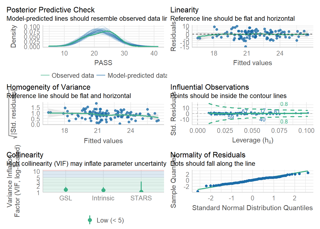

Although the bottom right plot for the normality of residuals is not quite capturing the peak of a normal distribution, there is nothing here to suggest there are any warning signs for our model.

With the findings and assumptions in order, we know what the real data set is telling us. Now, it is time to create a synthetic data set using the synthpop package to see how close it replicates the features.

2.3 Synthesise with `synthpop`

The synthpop package (Nowok et al., 2016) aims to mimic observed data and preserve the relationship between variables. The authors developed the package to work around limitations when working with the vast data coming from national statistical agencies. These population level data sets can provide important insights, but the granularity of the data rightly leads to privacy concerns about how identifiable the participants are, restricting access to the data. Working with higher education data, we can face similar concerns. We have access to student level data which can provide important insights, but we often cannot access or share that data because of confidentiality constraints. This is where synthetic data can be useful.

Packages like synthpop attempt to reconstruct the data set by sampling from probability distributions relevant to the type of data you are working on. This means the properties of the variables and relationships between them are retained as closely as possible. Sometimes this is more or less accurate, but we will explore factors to keep in mind later on.

2.3.1 Preparing the data set

Before creating a synthetic data set it is important to check your data to determine the number and type of variables, as well as how much missing data you have (if any) and you can do so using the codebook.syn() function.

codebook.syn(real_data)

## $tab
##           variable     class nmiss perctmiss ndistinct details
## 1              age   numeric     0         0        16        
## 2           gender character     0         0         4        
## 3 degree_programme character     0         0         4        
## 4              GSL   numeric     0         0        24        
## 5        Intrinsic   numeric     0         0        18        
## 6            STARS   numeric     0         0        25        
## 7             PASS   numeric     0         0        20        
## 
## $labs
## NULL

Whilst this output might look useful, it's actually missing a lot of information and that's because both the dataset and the individual variables are not quite in the right format.

The first step is to convert the object to a data frame. As we used the "tidyverse" family of packages, the data were saved as something called a tibble. Tibbles are similar to data frames, but have a few tweaks to work better in the tidyverse (see the tibble chapter in the R for Data Science book; Wickham & Grolemund, 2017). Although tibbles can be useful within the tidyverse framework, they can occasionally cause problems. We found this the hard way when writing this tutorial as if you try and use the data without converting it to a data frame, you get a cryptic error message Error in tab.obs[[i]] + tab.syn[[i]] : non-conformable array that took us an hour or so to figure out. It was only after reading a forum highlighting tibbles caused a similar problem for another package that we tried converting it to a data frame first which solved the issue.

The second step is to ensure all character variables are set to factors because whilst the data in these columns is text data, it's more informative than that as the text represents different categories. When creating the synthetic data set, the function works out a probability distribution using the original data, so setting characters to factors establishes the number of unique groups per variable.

# Resave real_data as a data frame instead of a tibble
real_data <- as.data.frame(real_data)

# Convert gender to a factor
real_data$gender <- as.factor(real_data$gender)

# Convert degree programme to a factor
real_data$degree_programme <- as.factor(real_data$degree_programme)

Now, when we repeat the codebook function, we get added details informing us of the number of levels per variable for factors and the data range for numeric variables. For this data set, we do not have any missing data, but if we did, the central columns would inform us of the number and percent of missing values, as this is also something that can be estimated as part of the synthetic data function.

codebook.syn(real_data)

## $tab
##           variable   class nmiss perctmiss ndistinct           details
## 1              age numeric     0         0        16    Range: 18 - 50
## 2           gender  factor     0         0         4 See table in labs
## 3 degree_programme  factor     0         0         4 See table in labs
## 4              GSL numeric     0         0        24  Range: 1.6 - 6.8
## 5        Intrinsic numeric     0         0        18 Range: 2.5 - 6.75
## 6            STARS numeric     0         0        25  Range: 1.875 - 5
## 7             PASS numeric     0         0        20     Range: 6 - 30
## 
## $labs
## $labs$gender
##                  label
## 1               Female
## 2                 Male
## 3           Non-binary
## 4 Prefer not to answer
## 
## $labs$degree_programme
##   label
## 1    BA
## 2   BSc
## 3    MA
## 4   MSc

2.3.2 Subset the data

Previously, we mentioned synthpop will match the features of the original data as closely as possible, but this can be more or less accurate. One factor associated with this is the ratio of the number of participants to the number of variables in the data set. A synthetic data set tries to retain the association between variables, so the larger the number of variables, the more combinations the function must consider. If you do not have enough participants, synthpop will provide a warning with the number of participants it recommends based on the number of variables in the data set. This is 100 + 10 * the number of variables. So, with two variables, they recommend 120 participants, eight variables 180 participants etc. If you have fewer participants than recommended, the estimation process might be less precise.

For this demonstration, we will first create a limited data set of two variables to show how it works, then scale it up to the full data set. In the following code, we set a seed to make the analyses reproducible. The function set.seed() controls the random number generator - if you're using any functions that use randomness, running set.seed() will ensure that you get the same result each time you run the function (in many cases this may not be what you want to do). Because the estimation for the synthetic data set is based on simulations, if you don't set a seed you won't get the same results as in this tutorial.

We know GSL was the strongest predictor in the original data, so we will limit the results to just predicting academic procrastination from GSL and then create a synthetic data set using the syn() function.

# Set a seed for reproducible analyses
my_seed <- 2018

# limit the real data to just two variables 
short_data <- real_data %>% 
  select(PASS, GSL)

# Save the synthetic data using the reproducible seed from above
synth_data <- syn(short_data, 
                   seed = my_seed)

## CAUTION: Your data set has fewer observations (111) than we advise.
## We suggest that there should be at least 120 observations
## (100 + 10 * no. of variables used in modelling the data).
## Please check your synthetic data carefully with functions
## compare(), utility.tab(), and utility.gen().
## 
## 
## Synthesis
## -----------
##  PASS GSL

Now, our synthetic data set is only saved as an object in the environment, but synthpop includes a function to save the new data in your current working directory. The following function takes the synthetic data object, what you would like the file to be called, and what file type you want it saved as:

write.syn(synth_data, 
          filename = "synthetic_Dunn_data", 
          filetype = "csv")

## Synthetic data exported as csv file(s).
## Information on synthetic data written to
##   C:/Users/staff/OneDrive - University of Glasgow/Teaching/psyteachR/scholaRship/book/synthesis_info_synthetic_Dunn_data.txt

If you ran the code to save the synthetic data set, you will see three new files in your working directory. There is an. RData object which you can reload into R. By choosing a .csv file, we also have a spreadsheet containing the data which we could analyse in other software or read into R. Finally, there is a .txt file with information on the synthetic data process like the name of the original data file, the seed you used, and the variables.

2.3.3 Compare data sets

Now we have our synthetic data, synthpop has some useful functions to compare your new data to the observed data. For example, you can compare the distribution of values between the two data sets to see how well it reconstructed the values. In the stat argument, you can choose either "counts" or "percents" to show the histogram as frequency or percentage of the values, depending on which you prefer to interpret.

compare(synth_data, # synthetic data object
        short_data, # original data
        stat = "counts") # Choice of counts or percents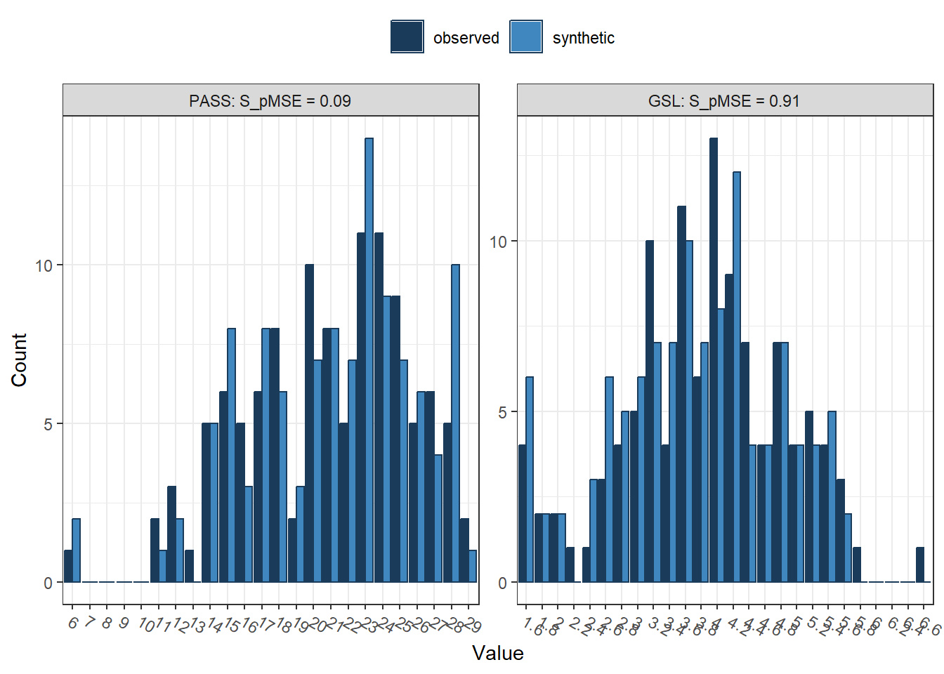

## 
## Comparing counts observed with synthetic
## 
## 
## Selected utility measures:
##          pMSE   S_pMSE df
## PASS 0.000207 0.091919  4
## GSL  0.002052 0.911044  4

We can see here two histograms for the limited selection of two variables. In dark blue, we have the frequency of observations from the observed data, and in light blue, we have the frequency of observations from the synthetic data. It is not a perfect match, with some observed values higher than synthetic, and some synthetic values higher than observed. It's never going to be perfect, so we are trying to capture the features as closely as possible, as different underlying distributions can produce the same relationships between variables.

After the histograms, we have the default settings for utility measures. These are statistics to summarise how closely the synthetic data compares to the observed data, assuming that the synthesis model is correct. The three default results are pMSE (propensity score mean-squared error), S_pMSE (a standardised measure of pMSE), and df (the degrees of freedom for the Chi-Square tests). There are many other utility measures which you can request using the utility.stats argument. To explore what measures are available, read the documentation by entering help("utility.tab") into the console.

If you want to fall down the statistics rabbit role, we refer you to Raab et al. (2021) and Snoke et al. (2018) who test different utility measures. For a brief overview, there are general/global or specific/narrow utility measures. Global measures attempt to capture how well the synthesis process reconstructs relationships across the whole data set rather than the result of one specific statistical model. In the output above, pMSE is one such measure. Propensity scores work by combining the two data sets and calculating the probability that an observation comes from the synthetic data. This means the propensity score mean-squared error (pMSE) measures the error associated with this process, with higher values meaning greater error. The closer to 0 the better, as this means the highest utility and it is hard to distinguish the two data sets. The further away from 0, the easier it is to distinguish the two data sets. Both values here are very small, so there should be nothing to worry about.

On the other hand, narrow measures compare the same models between data sets, such as how closely regression coefficients are replicated. The lm.synds() function from synthpop creates a linear model using the synthetic data sets, which you can then refit using the observed data to compare how different they are.

In the following code, we first create a simple linear regression model using PASS as the outcome and GSL as the single predictor. We save this as an object and use the compare() function from before.

# Linear model equivalent in synthetic data, one outcome and one predictor
s_lm <- lm.synds(PASS ~ GSL,
                 data = synth_data)

compare(s_lm, # saved object from above for lm applied to synthetic data
        short_data) # original data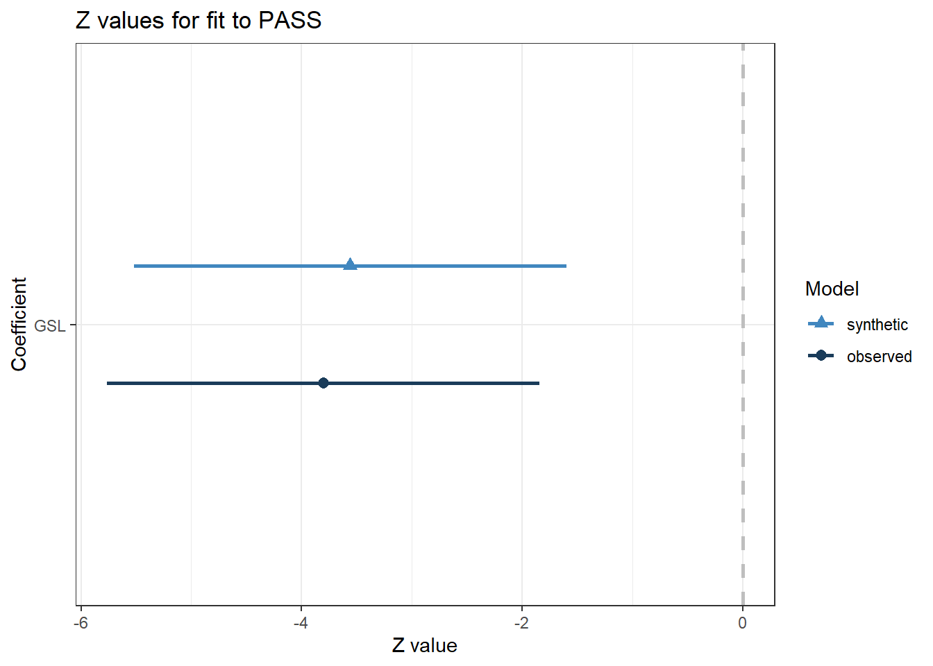

## 
## Call used to fit models to the data:
## lm.synds(formula = PASS ~ GSL, data = synth_data)
## 
## Differences between results based on synthetic and observed data:
##             Synthetic  Observed       Diff Std. coef diff CI overlap
## (Intercept) 27.856804 28.319159 -0.4623549     -0.2619675  0.9331703
## GSL         -1.497014 -1.598289  0.1012751      0.2409324  0.9385365
## 
## Measures for one synthesis and 2 coefficients
## Mean confidence interval overlap:  0.9358534
## Mean absolute std. coef diff:  0.25145
## 
## Mahalanobis distance ratio for lack-of-fit (target 1.0): 0.04
## Lack-of-fit test: 0.07152817; p-value 0.9649 for test that synthesis model is
## compatible with a chi-squared test with 2 degrees of freedom.
## 
## Confidence interval plot:

There is a bunch of output to dissect here, so we will start with the plot for a visual overview. Similar to the last compare() output, the observed data are displayed in dark blue and the synthetic data are displayed in light blue. The plot here shows the point estimate and confidence interval for the regression coefficient as a Z value. Visually, it looks pretty good. The synthetic data estimate is slightly smaller, but the confidence intervals largely overlap.

Now we have an initial impression, let's break down the output table. After informing you of the model you fitted, we have a summary of the model coefficients for the synthetic and observed data, the difference between them, and how much the confidence intervals overlap. For the intercept, there is a difference of -0.46 and for the GSL coefficient, a difference of 0.10. These are quite small, but keep in mind they are in the original units of measurement, so you will need to interpret the differences relative to the measures. Reinforcing our visual interpretation, the confidence intervals largely overlap, with approximately 93% coverage for both parameters.

Finally, we have a Chi-Square test which assumes the synthetic data model is compatible with the observed data model. In essence, the null hypothesis is that there is no difference between the two models. Acknowledging the limitations of null hypothesis significance testing, the smaller the p-value, the more incompatible the two models are. The p-value here is close to 1, suggesting there is not a significant difference between the two models. If the p-value was much smaller, such as below the traditional threshold of .05, we would suspect the synthetic data process did not capture the relationships in the observed data.

To summarise the smaller selection procedure, we limited the data set to two variables: predicting PASS from GSL scores. We created a synthetic data set using the synthpop package and explored general and narrow utility measures. Both types of measures showed the synthetic data set did a good job of capturing the properties of the observed data. This means we could share the synthetic data set if we had concerns about sharing the original observed data set. Just remember to clearly label the synthetic data set as a fake data set and inform readers this has replaced your observed data.

2.3.4 Full data set

Now we have taken a close look at a limited selection of variables, let's scale things up to see what synthpop looks like with more variable types and more relationships to consider. We will go back to using the original real_data file with all seven variables. The first step is using the syn() function again to create a new synthetic data set. We already processed this data set before reducing the number of variables, so remember to check if you are using a tibble and whether character variables need converting to factors.

synth_data2 <- syn(real_data, # return to using the original larger data set
                   seed = my_seed) # use same seed as above

## CAUTION: Your data set has fewer observations (111) than we advise.
## We suggest that there should be at least 170 observations
## (100 + 10 * no. of variables used in modelling the data).
## Please check your synthetic data carefully with functions
## compare(), utility.tab(), and utility.gen().
## 
## 
## Synthesis
## -----------
##  age gender degree_programme GSL Intrinsic STARS PASS

We are working with the same amount of data from 111 participants but trying to reconstruct more variables. Remember the synthetic data process is based on sampling from an appropriate probability distribution, so the package recommends a minimum number of participants (100 + 10 * the number of predictors). In the smaller selection, we were close to this recommendation as two predictors should have at least 120 participants. However, for the larger selection, we are further away from the recommendation as we should now have at least 170 participants. Keep this in mind when checking the utility measures.

Next, compare the two data sets to see how close we reconstructed the variables:

compare(synth_data2, 
        real_data, 
        stat = "counts")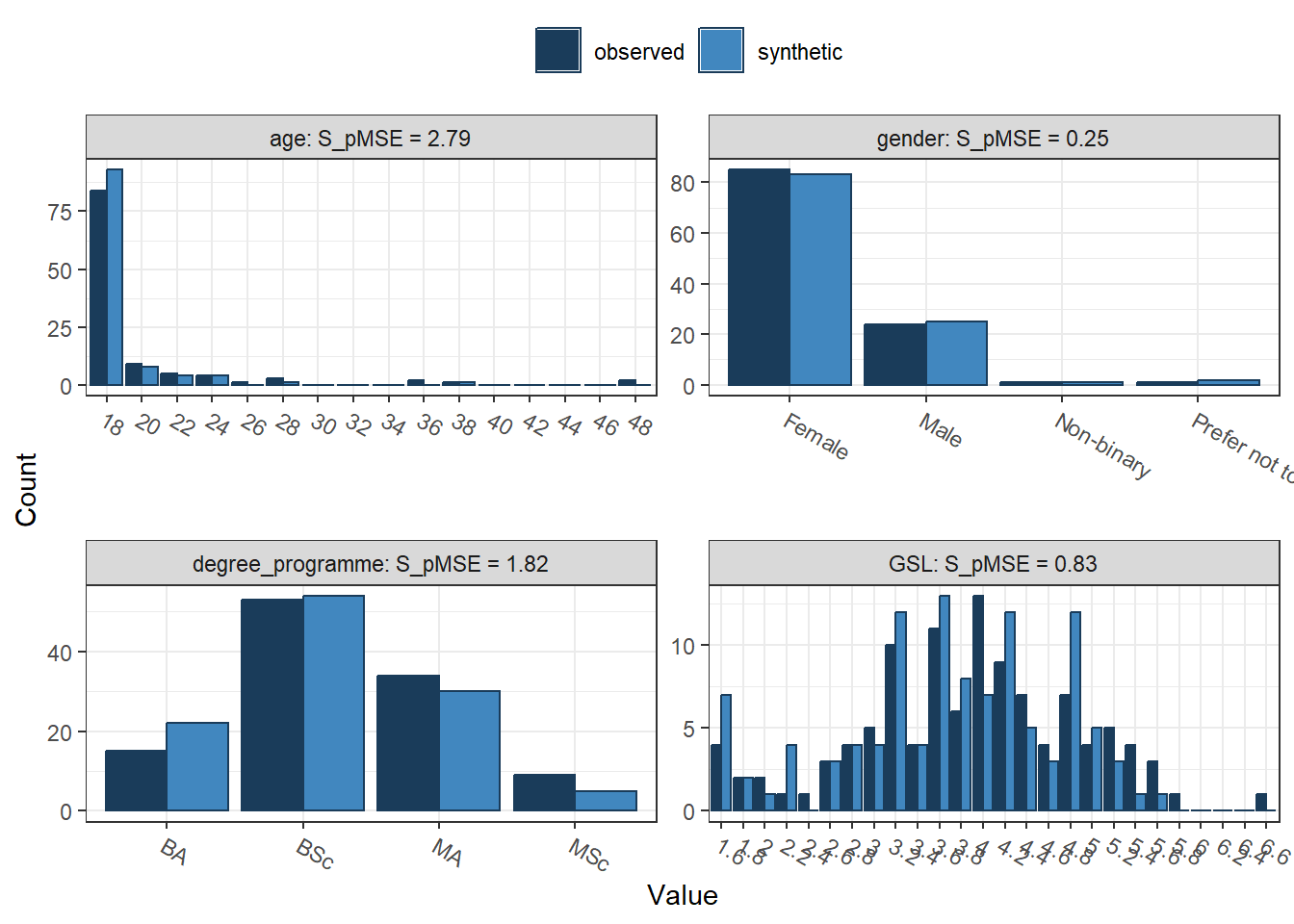

## 
## Comparing counts observed with synthetic
## 
## Press return for next variable(s): 
## 
## Selected utility measures:
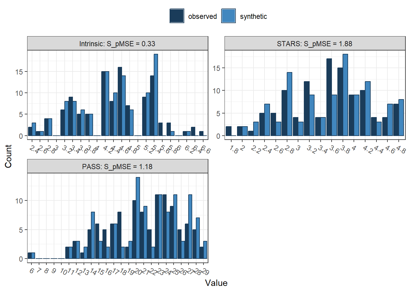
##                      pMSE   S_pMSE df
## age              0.003145 2.792530  2
## gender           0.000425 0.251701  3
## degree_programme 0.003070 1.817685  3
## GSL              0.001869 0.829618  4
## Intrinsic        0.000741 0.329097  4
## STARS            0.004231 1.878619  4
## PASS             0.002649 1.175969  4

The output here is longer since we now have seven variables to reconstruct instead of our smaller selection of two. We can also see what character variables look like since the smaller selection only contained two numeric variables. We have some demographic information we omitted for the smaller selection, so we can now see age, gender, and the participant's degree programme.

Below, we then have our variables of interest and what we will use next in multiple linear regression, using PASS (academic procrastination) as our outcome and three predictors of intrinsic motivation, GSL (general strategies for learning), and STARS (statistics and test anxiety). The final table is our general utility measures to see how well the synthetic data set captured the features of the observed data set. Remember pMSE is the error associated with classifying the data as coming from the synthetic or observed data set, with values further from 0 indicating greater error.

We will use the same function as before to create a linear model with the synthetic data set, then use the compare() function to see how the same model performs under each data set for our narrow utility measures:

# Second linear model using the full three predictors
s_lm2 <- lm.synds(PASS ~ GSL + Intrinsic + STARS,
                 data = synth_data2)

(synth_compare2 <- compare(s_lm2, # New full multiple linear regression model
        real_data)) # Full observed data file with our 7 variables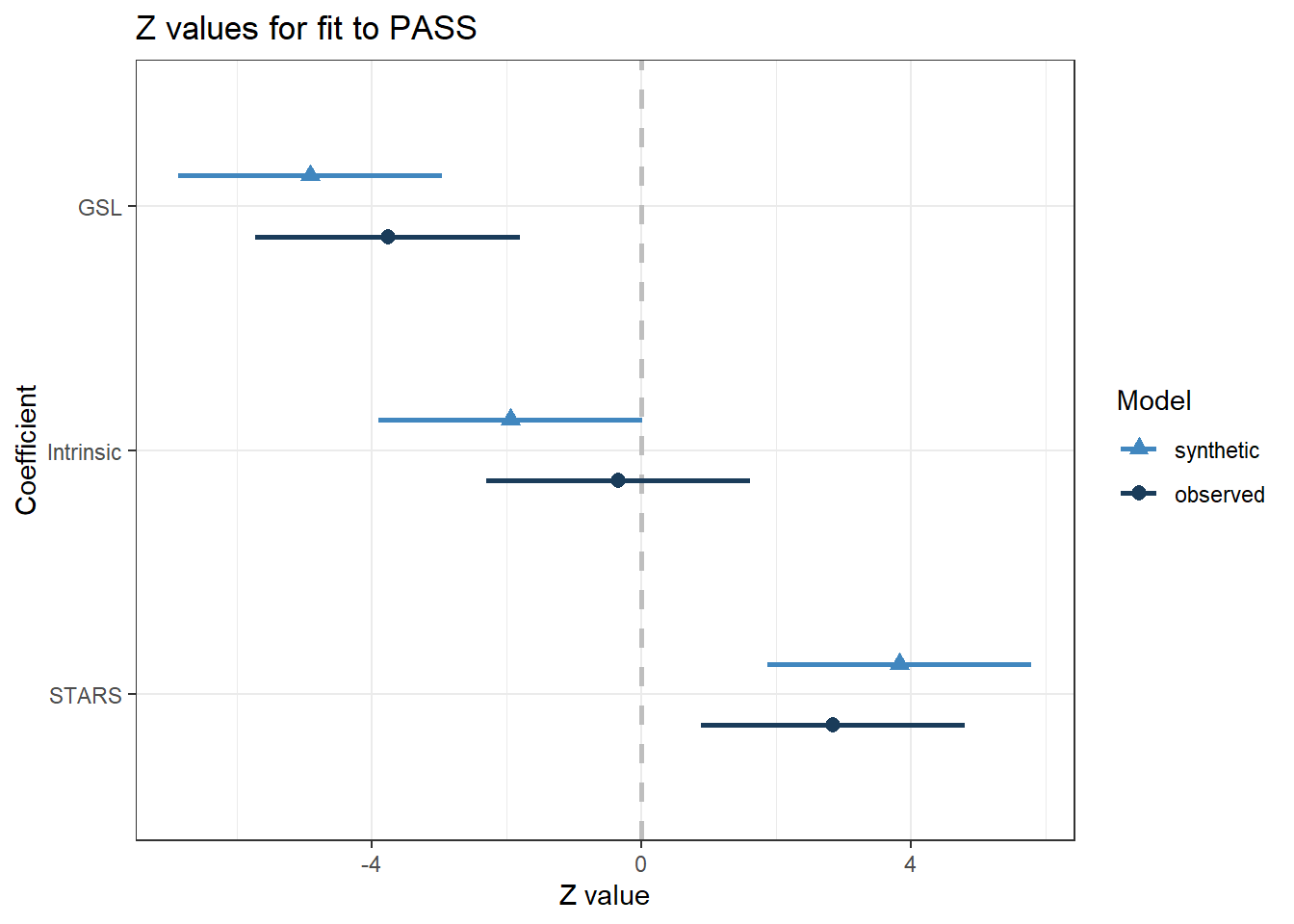

## 
## Call used to fit models to the data:
## lm.synds(formula = PASS ~ GSL + Intrinsic + STARS, data = synth_data2)
## 
## Differences between results based on synthetic and observed data:
##             Synthetic   Observed       Diff Std. coef diff CI overlap
## (Intercept) 27.316140 23.6386257  3.6775144      1.2230587  0.6879895
## GSL         -2.308385 -1.7676992 -0.5406860     -1.1508323  0.7064149
## Intrinsic   -1.002581 -0.1780281 -0.8245529     -1.5979280  0.5923578
## STARS        2.280006  1.6926311  0.5873745      0.9853746  0.7486243
## 
## Measures for one synthesis and 4 coefficients
## Mean confidence interval overlap:  0.6838466
## Mean absolute std. coef diff:  1.239298
## 
## Mahalanobis distance ratio for lack-of-fit (target 1.0): 1.92
## Lack-of-fit test: 7.683872; p-value 0.1039 for test that synthesis model is
## compatible with a chi-squared test with 4 degrees of freedom.
## 
## Confidence interval plot:

Starting again with a visual interpretation, the synthetic (light blue) and observed (dark blue) estimates are pretty close. GSL is a strong negative predictor, STARS is a moderate positive predictor, and intrinsic motivation is a weak predictor of PASS hovering around zero. The confidence intervals do not overlap quite as closely as for the smaller selection, but we will look at the precise statistics in a moment.

Moving to the table of estimates, we now have four parameters to check. We have the coefficients for the synthetic data set, observed data set, and the difference between them. Remember these values are unstandardised in the original units of measurement, so judge the differences as relative. Compared to the smaller selection, it had a harder time reconstructing the intercept, but the performance is OK for the three predictors. Supporting our visual inspection, the confidence interval coverage is lower than the smaller selection, but still captures the main features. The intrinsic motivation interval is the worst, while the STARS interval is the best. Now we have more parameters, it can also be helpful to look at the mean overlap across all confidence intervals, which was 68% in this case. The poorer performance is probably due to the smaller than recommended sample size compared to the smaller selection.

Finally, we can look at the Chi-Square test which assumes the synthetic data model is compatible with the observed data model. Smaller p-values suggest there is greater incompatibility between the two models. For the larger selection, it is also not statistically significant, suggesting narrow utility performance is not ideal, but it is not too inconsistent with the observed data.

2.4 Summary

In this tutorial, we explored how to create synthetic data sets in the context of the scholarship of teaching and learning. We often work with sensitive data or risk the anonymity of participants which may prevent us from accessing or sharing data. Open scholarship practices recognise the role and value of sharing research data, so synthetic data sets can provide a useful compromise between our scientific and ethical responsibilities.

We created synthetic data sets of a smaller and larger selection of variables from an unpublished replication attempt of Dunn (2014). When assessing how well the synthetic data reconstructs the observed data, there are general and narrow utility measures. General utility measures include statistics like pMSE (propensity score mean-squared error), whereas narrow utility measures include comparing model parameters like the regression coefficient and confidence interval. We saw how performance was worse when there was greater mismatch between the recommended and actual sample size, so keep the package recommendations in mind when creating your own synthetic data.

We tried to provide a relatively non-technical introduction to synthetic data sets which are more common in the world of statistical agencies or large granular data sets which increase the risk of re-identification. For further resources, we recommend the primer by Quintana (2020) who included additional sections exploring how different levels of skew and missing data affect the synthetic data process. For more technical details, we recommend the original package article by Nowok et al. (2016) and the synthpop website includes vignettes and a list of resources for learning more about synthetic data.

As a final remember, always include a label and instructions informing readers when you provide synthetic data, so they do not mistake it for the real observed data.

2.5 References

Meyer, M. N. (2018). Practical Tips for Ethical Data Sharing. Advances in Methods and Practices in Psychological Science, 1(1), 131–144. https://doi.org/10.1177/2515245917747656

Nowok, B., Raab, G. M., & Dibben, C. (2016). synthpop: Bespoke Creation of Synthetic Data in R. Journal of Statistical Software, 74, 1–26. https://doi.org/10.18637/jss.v074.i11

Quintana, D. S. (2020). A synthetic dataset primer for the biobehavioural sciences to promote reproducibility and hypothesis generation. ELife, 9, e53275. https://doi.org/10.7554/eLife.53275

Raab, G. M., Nowok, B., & Dibben, C. (2021). Assessing, visualizing and improving the utility of synthetic data (arXiv:2109.12717). arXiv. https://doi.org/10.48550/arXiv.2109.12717

Snoke, J., Raab, G. M., Nowok, B., Dibben, C., & Slavkovic, A. (2018). General and specific utility measures for synthetic data. Journal of the Royal Statistical Society: Series A (Statistics in Society), 181(3), 663–688. https://doi.org/10.1111/rssa.12358

Wickham, H. & Grolemund, G. (2017). R for Data Science. O'Reilly.

1 Introduction

3 Moodle Assignment submission reports